- Select Open in the File menu (or click on
 in the main Toolbar) to display the File Open box. Navigate to the Peranso Tutorials 9 folder. To do so, first locate your My Documents folder (typically C:\Users\<your_user_name>\Documents). In there is a subfolder Peranso, then select the subfolder Tutorials. Finally, select the folder 9. Finding extrema in observations. Select the file Light curve B1 and click the Open button. in the main Toolbar) to display the File Open box. Navigate to the Peranso Tutorials 9 folder. To do so, first locate your My Documents folder (typically C:\Users\<your_user_name>\Documents). In there is a subfolder Peranso, then select the subfolder Tutorials. Finally, select the folder 9. Finding extrema in observations. Select the file Light curve B1 and click the Open button.
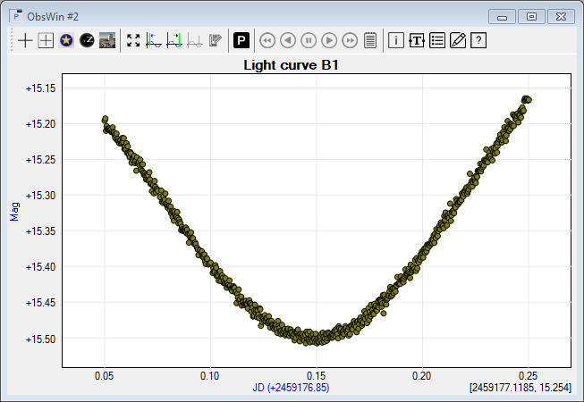
- The new ObsWin with Light curve B1 contains pseudo-observations which have been generated using a normal bell curve generation function, with the ToM being close to the JD 2,459,177.0 point. We furthermore added a linear function to make the curve asymmetric. The difference between minimum and maximum magnitude was set to about 0.3 magnitude, and the interval between observations was set at 0.0003 days. Finally, we also added noise to the light curve.
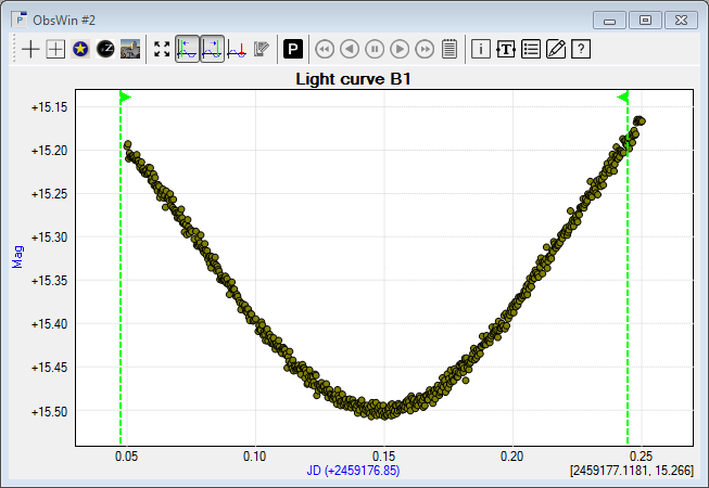
- We will now determine the Time of Minimum (ToM) using the Polynomial fit method. We first have to mark the X-axis interval of the light curve where the Polynomial fit should operate. We do this by using a Left Margin cursor and Right Margin cursor. The margin cursor section explains how to set the cursors.
In general, we recommend to position the margin cursors such that they are symmetric with the assumed location of the ToM in the middle. We also recommend to include as many observations as possible in the interval. However, one has to avoid parts of the light curve showing local minima or maxima (different from the minimum you are looking for). In other words, there should be only one minimum or maximum in the marked interval.
- Then click the Lightcurve Workbench button
 in the ObsWin toolbar. This brings up the Lightcurve Workbench box. Select the Polynomial fit tab. In the section Add polynomial, set Degree to 7. Click the Add button. This will display a 7-th degree polynomial, fitted through the light curve observations (solid blue line). The Polynomial is also added to the table in the Lightcurve Workbench. in the ObsWin toolbar. This brings up the Lightcurve Workbench box. Select the Polynomial fit tab. In the section Add polynomial, set Degree to 7. Click the Add button. This will display a 7-th degree polynomial, fitted through the light curve observations (solid blue line). The Polynomial is also added to the table in the Lightcurve Workbench.
Click the Calculate extremum button. This draws a Polynomial Extremum indicator at the calculated ToM (dotted blue line). The ToM value is shown next to the indicator and also in the table of the Lightcurve Workbench. Additionally, the corresponding calculated brightness value is displayed.
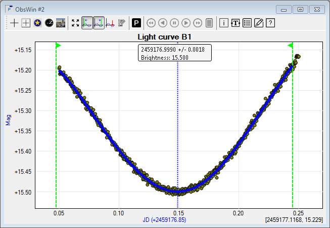

We obtain a measured ToM value of JD = 2,459,176.9991 +/- 0.0017. Note that the 'correct' ToM for this synthetic light curve is 2,459,177.0. This is within the interval of our measured ToM, and hence a good result. The addition (N=632) indicates that 632 observations have been used for the polynomial fit and extremum calculations.
Advanced exercise #1
With both Observations Windows still open, let's now calculate the ToM for the first ObsWin using the Polynomial fit method and compare it with the Kwee-van Woerden ToM. Using a 7-th degree polynomial we obtain a measured ToM value of 2,459,147.1009 +/- 0.0028. This interval still contains the correct ToM, but has a larger (and likely more realistic) error value than the Kwee-van Woerden method. Zoom in closely on the ToM with both extremum indicators visible. Then use the Measurement indicator to draw a line of 'length' 0.0028 near the ToM. It gives you an idea of the error interval calculated by the Polynomial fit extremum.
Advanced exercise #2
The second ObsWin still shows the ToM calculated with the Polynomial fit method. Let's now calculate the ToM using the Kwee-van Woerden method and compare it with the Polynomial fit ToM. We obtain a measured ToM value of 2,459,176.9978 +/- 0.0001. This interval no longer contains the correct ToM, and again shows that the error value reported by the Kwee-van Woerden method is too optimistic.
|