|
In the previous section, we learned to auto-search for multiple periods in the RX Cap light curve and found two dominant periods at 67.97 days and 140.37 days. In this section, we will manually search for periods. Auto-search is the recommended method to look for multiple periods using the CLEANest Workbench. However, if you want to explore additional search capabilities, you might decide to opt for the manual search.
- Close all windows from the previous section of this tutorial, except for the ObsWin. Open the Period determination box and make sure that the Range values are 50 (Start), 200 (End) and 2500 (Steps). Select the CLEANest (Foster) Method and click Apply.
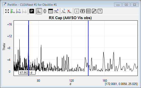
- This shows the same PerWin as found in the previous section of this tutorial. Click the CLEANest Workbench button in the PwerWin toolbar. In this part of the tutorial, we will focus on the Manual search section of the tool.
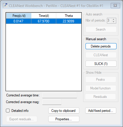
- The strongest peak in the Peaks Table appears at a period of 67.96 days with a power (theta) value of 22.86. Since we are not yet interested in other periods, we delete all entries of the Peaks Table, except for the first one. This is done by selecting the corresponding rows in the table and by then pushing the Delete periods button.

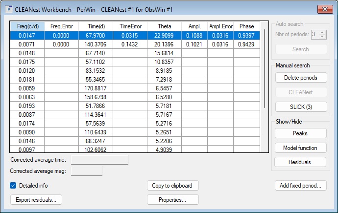
Whenever one runs a Fourier analysis, it is possible that the peak signal may not be the precise frequency actually detected in the data set, because the sampled frequencies tested might be offset slightly from the true signals. We use the CLEANest button to perform this refinement. First select the remaining entry in the Peaks Table, and then press the CLEANest button. The Peak Table gets updated and you will see that the first period has been displaced in the table, and that a new entry appears above it, with period 67.97 days and a power of 22.91.
Delete the old (second) entry from the Peaks Table, using the Delete Periods button.
- We will now create the CLEANest(1) spectrum, or more precisely SLICK(1) spectrum. This is done by subtracting the peak from the time series data, and by doing a Fourier transform of the residual spectrum. This operation is accomplished with the SLICK button. First select the strongest peak (period 67.97 d) in the Peaks Table, and then click the SLICK(1) button.
Once the Fourier transform of the residual spectrum has been completed, the Peaks Table is automatically updated to indicate the new peaks of the residual spectrum. The entry with period 67.97 d is maintained.
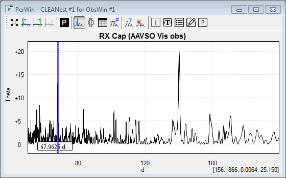
- Select that entry and click the Peaks button in the Show/Hide section to draw the discrete spectrum peak at a period of 67.97 d. The corresponding entry in the Peaks Table is highlighted, to indicate the existence of a discrete spectrum peak.
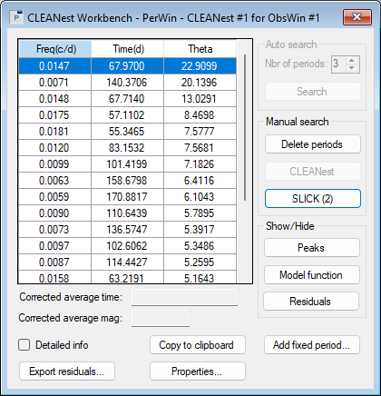
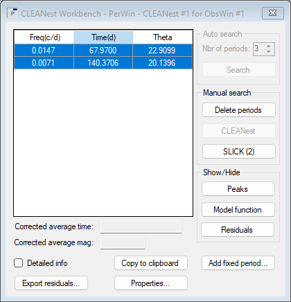
- We continue with the calculation of the SLICK(2) spectrum. This is done by subtracting the two best peaks from the time-series data, and by doing a Fourier transform of the residual spectrum. This operation is accomplished by removing all peaks from the Peaks Table, except for the 2 top ones. Select those 2 peaks (the one at period 67.97 d, and the one at 140.37 d) in the Peaks Table and click the SLICK(2) button.
- Once the Fourier transform of the residual spectrum has been completed, select the 2 peaks in the Peaks Table and press the Peaks button to create the SLICK(2) spectrum.
- The third entry in the Peaks Table shows a period at 67.71 days, which is nearly identical to the one of 67.97 days and therefore is not a true (new) period. The fourth entry shows a period at 57.11 days. However, its power level of 11 is half of the power level of the two dominant peaks, and therefore no longer 'significant'. We can safely conclude that RX Cap has two periods.
- Select the Detailed Info option to expand the CLEANest Workbench box. A number of new columns appear : amplitude and phase of the peaks, and error values for frequency, period and amplitude.
- Finally, create a Spectral Window (explained in Tutorial 2) to confirm that the periods found in this section are not an artifact of the observing rate.
Conclusions
RX Cap is a multi-period system with periods :
P0 : 67.97 +/- 0.03 d
P1 : 140.37 +/- 0.14 d
This is in excellent agreement with the published values of 67.93 and 140.33 days in John R. Percy's paper
Advanced exercise
Use the Prewhitening approach, explained in Tutorial 3, in combination with the Lomb-Scargle GLS method, to check for the presence of multiple periods in RX Cap. You will find a first period at 67.96 days. Doing a prewhitening shows a second period at 140.37 days, which is confirming our above findings. Doing a third prewhitening will again show the 67.71 days period, which we previously rejected. Doing a fourth prewhitening shows a Lomb-Scargle GLS PerWin in which the False Alarm Probability FAP indicators (displayed as dashed green-orange-red lines) clearly indicate that no significant periods are left.
|