- We are used to look at Period Windows in a graphical way, as we have done so far in all previous tutorials. Peranso also offers the possibility to textually display the values used to draw the Period Window. Click the Textual View button
 in the PerWin toolbar to bring up the Textual View box. in the PerWin toolbar to bring up the Textual View box.
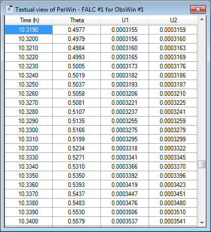
- The Textual View form contains a table in which one row has an highlighted Time cell. This is the row with the best period Peranso could find (which is not necessarily the correct period). It is the period with a minimum Theta (RMS) value. That value is the RMS (Root-Mean-Square) dispersion, in units of the a priori estimated uncertainty (thus, 1.0 means the fit is exactly as good as you estimated the default magnitude error value to be).
Remark : it is recommended to work with dispersion values > 1.0, i.e. better than the formal noise in the data.
Each row in the table displays the value of the period [Time(h)], the Theta RMS dispersion [Theta] , and two columns of fit uncertainty [U1] [U2] in units of magnitude.
- The first of the two columns of fit uncertainty [U1] is the formal uncertainty of the fitted curve, that is, the RMS fit dispersion divided by sqrt[(N)(N-K)], where N is the number of observations, and K is the number of solution constants1. The second column [U2] is the same, except divided by sqrt[(N)(N-K-1)].
- The difference between the values in the the two columns is a formal measure of significance of changing the solution. That is: if you force the solution off from the minimum value of dispersion by an amount that raises the dispersion in the U1 column to be equal to the value in the U2 column at minimum, then you are “one sigma” off of the least squares solution.
Example. For a period of 10.319 hours, the U1 value is 0.0003155 and the U2 value is 0.0003159. The latter is the "U2 value at minimum". Now have a look at the row just above and below the highlighted row. Compare their U1 values to the "U2 value at minimum". Both have a U1 value below the "U2 value at minimum", so both periods are less than one sigma off. We now move one row further up and further down, arriving resp. at 10.317 and 10.321 hours. Their U1 values are identical (by coincidence) at 0.0003160, which is just above the "U2 value at minimum". So, we have reached the one sigma offset. The difference between these periods and the minimum period is 10.319 - 10.317 = 0.002 h. We therefore infer that the formal uncertainty of the period determined is +/- 0.002 hours, in agreement with our conclusion from the previous section.
We will see in Part 2 that we can further try to refine this period, by running an Harmonic Order Scan.
(1) The number of solution constants is (2 * N + NbrObsSets), where N is the harmonic order and NbrObsSets is the number of ObsSets in your light curve. Example : if N = 4 and you use 4 ObsSets, then the number of solution constants is 12. You should always ensure that the total number of observations in your light curve is at least double of the number of solution constants.
|