- The light curve from previous section shows a few spurious data points, which we will ignore in this tutorial. It also contains a central gap with no observations.
Let's zoom in on some parts of the light curve to find out if we can detect the possible signature of an exoplanet transit. Let's do so on the left part of the light curve, for example between JD 2,458,325 and JD 2,458,332.8. The ObsWin will look similar to the below one:
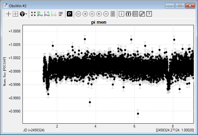
- We notice two "dips" in the light curve: one near JD 2,458,325.49 and one near JD 2,458,331.79. The difference between both dips is about 6.3 days. If we now zoom in on other sections of the light curve, we will find additional dips separated by approx. 6.3 days.
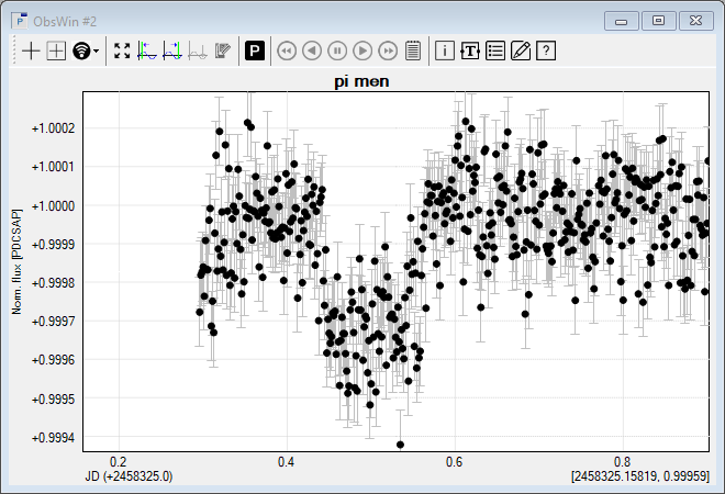
Furthermore, if we zoom in on one of the dips, we notice that the dip profile indeed resembles an exoplanet transit. For instance, zooming in on the first dip produces the below light curve:
- Peranso offers a particularly effective method to analyze stellar photometric time series in search for periodic transits by exoplanets, called EEBLS (Edge Enhanced Box-fitting Least Squares). Peranso allows calculating and visualizing the EEBLS frequency spectrum, folding of the time series over the most dominant EEBLS period, calculating the epoch of mid-transit events, the transit depth and duration, etc. In addition, Peranso graphically displays the fit obtained by the EEBLS method. EEBLS is explained in more detail in Tutorial 6.
- Click the Period Determination button in the ObsWin toolbar and select the EEBLS method. We select Days and Time and use a Range going from 5 to 7 days (as we know that the likely transit period is ~6.3 days). We immediately select a high number of Steps, 5000. In the Additional parameters section, we select 1000 bins in Nb, 0.01 as Min frac. transit length and 0.1 as Max frac. transit length.
Click Apply to start the EEBLS calculation. The EEBLS algorithm aims to find the best model with estimators for the transit period, depth and length, as well as the epoch of mid transit and the phase of ingress and egress.
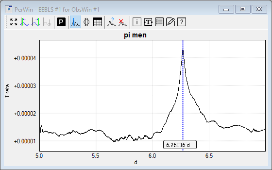
- This creates a Period Window (PerWin) with the EEBLS spectrum. Using the PerWin Info box, we note that the dominant period is 6.26836 +/- 0.05748 days. The dominant period is the transit period of exoplanet Pi Mensae c, and is in excellent agreement with the literature value we quoted at the start of this tutorial.
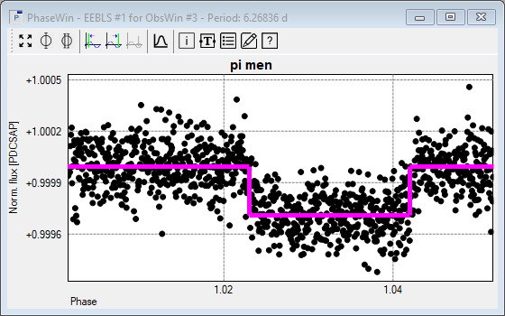
- The Period Window Info box shows that the transit duration is 0.145 d, which is a bit longer than the literature value. Finally, let's graphically display the fit obtained by the EEBLS method. To do so, we select PhaseWin at Frequency Cursor value in the Period analysis menu (or click on
 in the PerWin toolbar). This creates a Phase Window showing the result of folding the Pi Mensae c time series data over the dominant period of 6.26836 d. Zoom in on the part of the PhaseWin showing the transit. in the PerWin toolbar). This creates a Phase Window showing the result of folding the Pi Mensae c time series data over the dominant period of 6.26836 d. Zoom in on the part of the PhaseWin showing the transit.
- Click the right mouse button anywhere in the plot area of the Phase Window to display a context menu. Select Show/hide EEBLS fit to graphically display the EEBLS fit in the PhaseWin. Selecting the same entry again will hide the EEBLS fit. Zoom in on the Phase Window to obtain a view similar to the one below.
|